
Deep Q-Learning with Keras and Gym
This blog post will demonstrate how deep reinforcement learning (deep Q-learning) can be implemented and applied to play a CartPole game using Keras and Gym, in less than 100 lines of code!
I’ll explain everything without requiring any prerequisite knowledge about reinforcement learning.
The code used for this article is on GitHub.
Reinforcement Learning
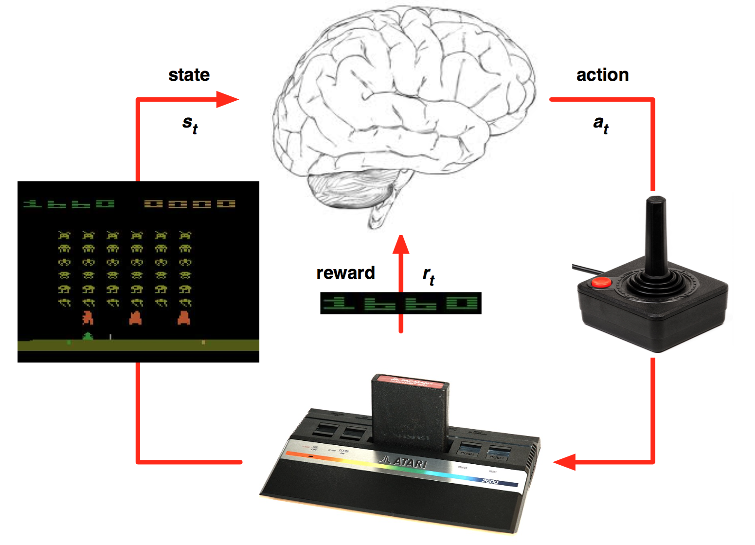
Reinforcement Learning is a type of machine learning that allows you to create AI agents that learn from the environment by interacting with it. Just like how we learn to ride a bicycle, this kind of AI learns by trial and error. As seen in the picture, the brain represents the AI agent, which acts on the environment. After each action, the agent receives the feedback. The feedback consists of the reward and next state of the environment. The reward is usually defined by a human. If we use the analogy of the bicycle, we can define reward as the distance from the original starting point.
## Deep Reinforcement Learning
Google’s DeepMind published its famous paper Playing Atari with Deep Reinforcement Learning, in which they introduced a new algorithm called Deep Q Network (DQN for short) in 2013. It demonstrated how an AI agent can learn to play games by just observing the screen without any prior information about those games. The result turned out to be pretty impressive. This paper opened the era of what is called ‘deep reinforcement learning’, a mix of deep learning and reinforcement learning.
Click to Watch: DeepMind’s Atari Player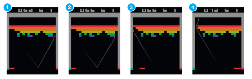
In Q-Learning Algorithm, there is a function called Q Function, which is used to approximate the reward based on a state. We call it Q(s,a), where Q is a function which calculates the expected future value from state s and action a. Similarly in Deep Q Network algorithm, we use a neural network to approximate the reward based on the state. We will discuss how this works in detail.
Cartpole Game
Usually, training an agent to play an Atari game takes a while (from few hours to a day). So we will make an agent to play a simpler game called CartPole, but using the same idea used in the paper.
CartPole is one of the simplest environments in OpenAI gym (a game simulator). As you can see in the animation from the top, the goal of CartPole is to balance a pole connected with one joint on top of a moving cart. Instead of pixel information, there are 4 kinds of information given by the state, such as angle of the pole and position of the cart. An agent can move the cart by performing a series of actions of 0 or 1 to the cart, pushing it left or right.
Gym makes interacting with the game environment really simple.
1 | next_state, reward, done, info = env.step(action) |
As we discussed above, action can be either 0 or 1. If we pass those numbers, env, which represents the game environment, will emit the results. done is a boolean value telling whether the game ended or not. The old stateinformation paired with action and next_state and reward is the information we need for training the agent.
## Implementing Simple Neural Network using Keras
This post is not about deep learning or neural net. So we will consider neural net as just a black box algorithm that approximately maps inputs to outputs. It is basically an algorithm that learns on the pairs of examples input and output data, detects some kind of patterns, and predicts the output based on an unseen input data. Though neural network itself is not the focus of this article, we should understand how it is used in the DQN algorithm.
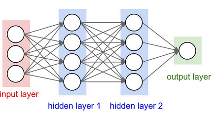
Note that the neural net we are going to use is similar to the diagram above. We will have one input layer that receives 4 information and 3 hidden layers. But we are going to have 2 nodes in the output layer since there are two buttons (0 and 1) for the game.
Keras makes it really simple to implement a basic neural network. The code below creates an empty neural net model. activation, loss and optimizer are the parameters that define the characteristics of the neural network, but we are not going to discuss it here.
1 | # Neural Net for Deep Q Learning |
In order for a neural net to understand and predict based on the environment data, we have to feed it the information. fit() method feeds input and output pairs to the model. Then the model will train on those data to approximate the output based on the input.
This training process makes the neural net to predict the reward value from a certain state.
1 | model.fit(state, reward_value, epochs=1, verbose=0) |
After training, the model now can predict the output from unseen input. When you call predict() function on the model, the model will predict the reward of current state based on the data you trained. Like so:
1 | prediction = model.predict(state) |
## Implementing Mini Deep Q Network (DQN)
Normally in games, the reward directly relates to the score of the game. Imagine a situation where the pole from CartPole game is tilted to the right. The expected future reward of pushing right button will then be higher than that of pushing the left button since it could yield higher score of the game as the pole survives longer.
In order to logically represent this intuition and train it, we need to express this as a formula that we can optimize on. The loss is just a value that indicates how far our prediction is from the actual target. For example, the prediction of the model could indicate that it sees more value in pushing the right button when in fact it can gain more reward by pushing the left button. We want to decrease this gap between the prediction and the target (loss). We will define our loss function as follows:
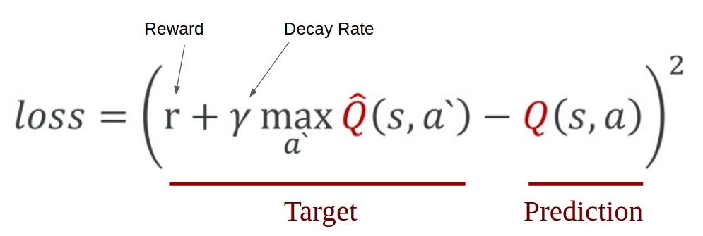
Mathematical representation of Q-learning from Taehoon Kim's slides
We first carry out an action a, and observe the reward r and resulting new state s`. Based on the result, we calculate the maximum target Q and then discount it so that the future reward is worth less than immediate reward (It is a same concept as interest rate for money. Immediate payment always worth more for same amount of money). Lastly, we add the current reward to the discounted future reward to get the target value. Subtracting our current prediction from the target gives the loss. Squaring this value allows us to punish the large loss value more and treat the negative values same as the positive values.
Keras takes care of the most of the difficult tasks for us. We just need to define our target. We can express the target in a magical one-liner in python.
1 | target = reward + gamma * np.amax(model.predict(next_state)) |
Keras does all the work of subtracting the target from the neural network output and squaring it. It also applies the learning rate we defined while creating the neural network model. This all happens inside the fit() function. This function decreases the gap between our prediction to target by the learning rate. The approximation of the Q-value converges to the true Q-value as we repeat the updating process. The loss will decrease and score will grow higher.
The most notable features of the DQN algorithm are memorize and replay methods. Both are pretty simple concepts. The original DQN architecture contains a several more tweaks for better training, but we are going to stick to a simpler version for now.
Memorize
One of the challenges for DQN is that neural network used in the algorithm tends to forget the previous experiences as it overwrites them with new experiences. So we need a list of previous experiences and observations to re-train the model with the previous experiences. We will call this array of experiences memory and use memorize() function to append state, action, reward, and next state to the memory.
In our example, the memory list will have a form of:
1 | memory = [(state, action, reward, next_state, done)...] |
And memorize function will simply store states, actions and resulting rewards to the memory like below:
1 | def memorize(self, state, action, reward, next_state, done): |
done is just a boolean that indicates if the state is the final state.
Simple right?
Replay
A method that trains the neural net with experiences in the memory is called replay(). First, we sample some experiences from the memory and call them minibath.
1 | minibatch = random.sample(self.memory, batch_size) |
The above code will make minibatch, which is just a randomly sampled elements of the memories of size batch_size. We set the batch size as 32 for this example.
To make the agent perform well in long-term, we need to take into account not only the immediate rewards but also the future rewards we are going to get. In order to do this, we are going to have a ‘discount rate’ or ‘gamma’. This way the agent will learn to maximize the discounted future reward based on the given state.
1 | # Sample minibatch from the memory |
## How The Agent Decides to Act
Our agent will randomly select its action at first by a certain percentage, called ‘exploration rate’ or ‘epsilon’. This is because at first, it is better for the agent to try all kinds of things before it starts to see the patterns. When it is not deciding the action randomly, the agent will predict the reward value based on the current state and pick the action that will give the highest reward. np.argmax() is the function that picks the highest value between two elements in the act_values[0].
1 | def act(self, state): |
act_values[0] looks like this: [0.67, 0.2], each numbers representing the reward of picking action 0 and 1. And argmax function picks the index with the highest value. In the example of [0.67, 0.2], argmax returns 0 because the value in the 0th index is the highest.
## Hyper Parameters
There are some parameters that have to be passed to a reinforcement learning agent. You will see these over and over again.
episodes- a number of games we want the agent to play.gamma- aka decay or discount rate, to calculate the future discounted reward.epsilon- aka exploration rate, this is the rate in which an agent randomly decides its action rather than prediction.epsilon_decay- we want to decrease the number of explorations as it gets good at playing games.epsilon_min- we want the agent to explore at least this amount.learning_rate- Determines how much neural net learns in each iteration.
## Putting It All Together: Coding The Deep Q-Learning Agent
I explained each part of the agent in the above. The code below implements everything we’ve talked about as a nice and clean class called DQNAgent.
1 | # Deep Q-learning Agent |
## Let's Train the Agent
The training part is even shorter. I’ll explain in the comments.
1 | if __name__ == "__main__": |
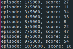
Result
In the beginning, the agent explores by acting randomly.
It goes through multiple phases of learning.
- The cart masters balancing the pole.
- But goes out of bounds, ending the game.
- It tries to move away from the bounds when it is too close to them, but drops the pole.
- The cart masters balancing and controlling the pole.
After several hundreds of episodes (took 10 min), it starts to learn how to maximize the score.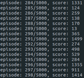
The final result is the birth of a skillful CartPole game player!
The code used for this article is on GitHub.. I added the saved weights for those who want to skip the training part.